
Polynomial division
1. Original procedure of the algorithm
If we divide two polynomials $f, g$ of one variable, we arrange them in the same way as two integers we want to divide.
- We put the divident $f$ and the divisor $g$ next to each other.
- We find the terms of both polynomials with the largest degree and divide them.
- We put the result $q_1$ of the division next to the divisor $g$ and then multiply $p = q_1 \cdot g$.
- We put the semi-result $p$ below the divident $f$ while respecting the vertical alignment of the terms of the same degree.
- We subtract $f_1 = f - p$ and put the polynomial $f_1$ below the expression $p$, again with respect to the vertical alignment of the terms of the same degree.
- We repeat the procedure with the polynomials $f_1, g$ and receive polynomials $f_2, f_3, \dots, f_n$, and $q_2, q_3, \dots, q_n$ respectively. The algorithm is finished when the polynomial $f_{ n + 1 }$ is of a lower degree than the divisor $g$.
- The sum $q = q_1 + q_2 + q_3 + \dots + q_n$ is the result of the division $f : g$ (so called quotient) with the remainder $f_{ n + 1 }$.
We add one specific example – division of two polynomials (Animation 1):
2. Proposals of adaptation
1. Consistent copying of all the expressions which occur during the computation:
Linear production of polynomials including a short description of each semi-result. See the example in the Lambda editor in Image 1:
Example 2: Polynomial division – linear computation
Link to a file with lambda extension:
polynomial_division_2_en.lambda
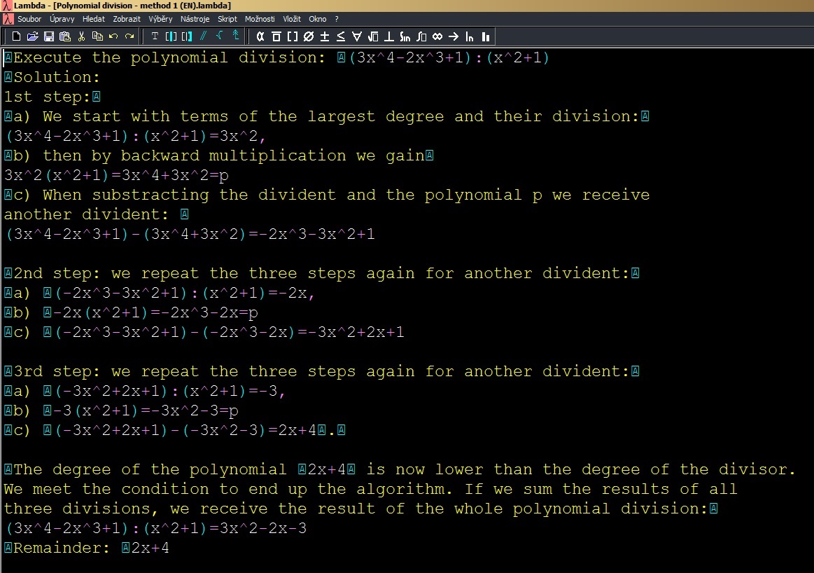 Image 1:
polynomial division – demonstration of linear computation including commentary
Image 1:
polynomial division – demonstration of linear computation including commentary
2. Entering the polynomials into a Spreadsheet using only their coefficients:
The first row is reserved for the powers of the divident, the divisor and the quotient, followed from left to right, each two polynomials are separated by an empty column. Other rows are determined for writing down the coefficients which should be located in the same columns as the power of the specific term. We put the polynomials $f_1, f_2, \dots, f_n, f_{ n + 1}$ below the divident. See the example of the computation in MS Excel in Image 2:
Example 3: Polynomial division using a spreadsheet
Link to a file with MS Excel extension:
polynomial_division_3_en.xls
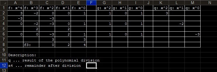 Image 2:
polynomial division, using the only coefficients in a spreadsheet to denote polynomials
Image 2:
polynomial division, using the only coefficients in a spreadsheet to denote polynomials
3. Entering all the polynomials into one (text) file, one below the other:
The method is based on the following fact: In every step of the algorithm, the blind student only works with two input polynomials. He/she executes a single operation with them and receives the third polynomial. Therefore, the idea of the adaptation is simple: the student should keep these polynomials together on three following lines. Then he can easily move between them using the keys down arrow or up arrow only once or twice. See the example of the procedure in the Lambda editor (Animation 2):
Example 4: Polynomial division in the Lambda editor
4. All the polynomials are organised in three files or sheets of a spreadsheet:
- We place the divident and the polynomials $f_1, f_2, \dots, f_n, f_{ n + 1}$ into the rows of the first file so that we respect their original arrangement set up according to the standard algorithm. If we use the spreadsheet we may describe all the polynomials only with their coefficients as it was done in the second method.
- We put the divisor into the second file (or sheet).
- In the third file (or sheet) there are the polynomials $q_1, q_2, \dots, q_n$ which give us the quotient $q = q_1 + q_2 + q_3 + \dots + q_n$.
During computation we can switch between these files (or sheets) by
pressing the key combination Alt+Tab (or Ctrl+PgUp,
Ctrl+PgDown) and modify them all except the divisor, whose value remains constant.
3. Discussion of pros and cons
We summarize the pros and cons of all the four methods of the polynomial division's adaptation.
The first method meets the requirement of the computation's comprehensibility. The whole procedure is understandable to the person responsible for supervising or evaluating the work of the blind person – there is no need for additional explanation. Unfortunately, it is not very economic ‐ the computation takes a lot of time and memory of the student. He works with the divisor very often, so he/she has to keep it in his memory or search for it in the previous text – which is very time-consuming. Even when preparing the final result he/she has to go through the whole text and pick up all the particular terms $q_1, q_2, \dots, q_n$.
The second method respects the original arrangement of the polynomials which is used when a sighted person performs the algorithm in the standard manner. So the procedure is understandable to the supervisor although he can be confused because only coefficients are used instead of the whole terms of the polynomials. However, the workshop participants discovered several disadvantages:
- Accessibility of the coefficients is not easy – blind students spend a lot of time moving between three objects and do not have an option to ignore specific values of the polynomials.
- Additionally, orientation is very difficult – the blind have to make sure very often which power corresponds to the coefficient they have actually reached.
- If they want to save some time, they are constantly occupied by holding semi-results in their memory as they are looking for a position where to insert them.
One of the workshop participants proposed a~possible solution of the problem described innbsp;item 2: "If the blind user could immediately get to know the power related to the actual coefficient, it would help him to orientate in the table, for example a simple script or macro which would substitute a lot of keystrokes when moving cursor to the first row and back.
José Enrique Fernández del Campo offered an adaptation very similar to our second method. His approach is more simple: blind students work only with two groups of coefficients. Prof. del Campo built his method on the fact that the divisor does not change during the computation so we can put the terms (not only coefficients) of the quotient below the powers of the divisor. This approach partially solves the problem described in item 1. The student follows only two groups of coefficients – the objects' accessibility during computation is easier. We provide an example of del Campo's method in the Lambda editor. To work with polynomials he uses the tool for matrix manipulation (Image 3):
Example 5: Polynomial division in Lambda editor
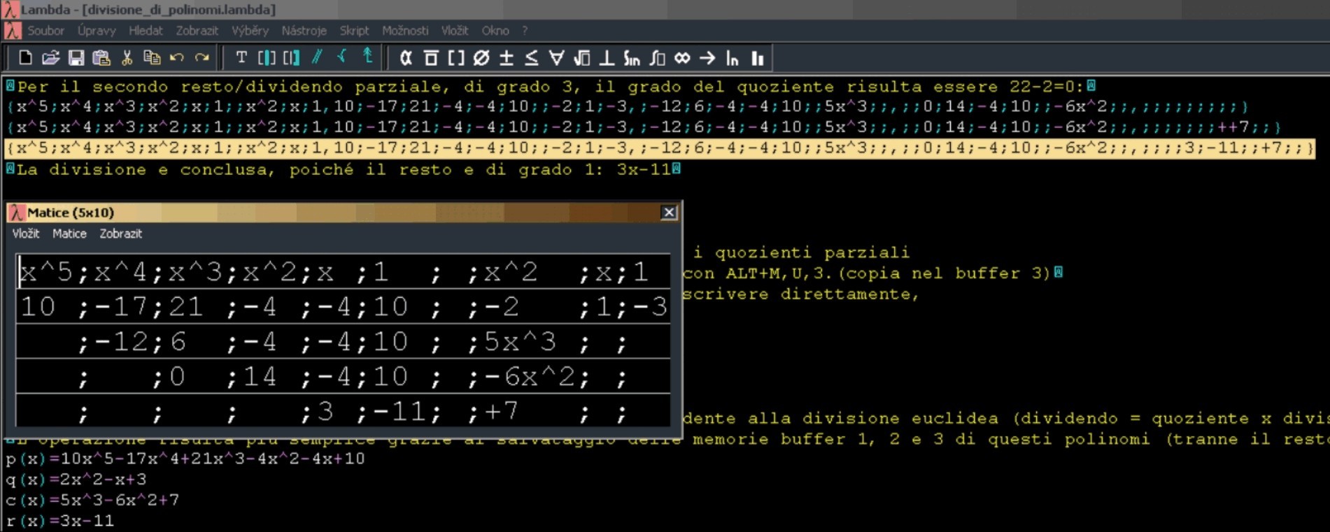 Image 3:
polynomial division in Lambda editor according to the proposal of Prof. del Camp
Image 3:
polynomial division in Lambda editor according to the proposal of Prof. del Camp
Let’s mention Cristian Bernareggi’s article called "Non-sequential Mathematical Notations in the LAMBDA System", in which he also deals with the adaptation of polynomial division. His proposal is nearly the same as that of Prof. del Campo. The only difference can be recognised in the manner of writing polynomials. Bernareggi uses coefficients only for the divident and the polynomials $f_1, f_2, \dots, f_n, f_{ n + 1}$, which are located one below the other. The divisor and the terms of the quotient are placed as whole expressions, not only represented by coefficients.
The participants of the workshop evaluated the third method as the most convenient. There is no question of the optimal access to objects we work with during the procedure. In every step of the computation we perform a certain mathematical operation with two polynomials and insert its result into a given position. Therefore it is good to have them as close as possible. At first, the blind student creates an empty line for inserting the result of the operation. Then he moves between two input polynomials by pressing only one key. He performs the operation very easily without occupying his memory too much and then saves the result above or below two actually processed polynomials. This approach also provides an easy access to objects which we will process in the following steps of the computation. The final inscription of the computation is not immediately understandable to the supervisor because it does not respect the original arrangement of objects we work with during the standard procedure of the algorithm. But if the student is consistent in writing all the polynomials including their names in front, then a short explanation at the beginning of the computation should be sufficient.
Finally the forth method offers the same advantage as the third one, that is the easy access to polynomials we actually work with. It is not very useful when the blind student wants to present the inscription of his/her computation to the supervisor. All the polynomials are divided into three files (or sheets), therefore the teacher evaluating the work of the blind student has to continuously switch between them, which is not comfortable for any sighted person. For this reason, the student should help his teacher and put the content of these three files (or sheets) into a single document after the whole computation has been done.